Charts

Charts are standalone kaxe.Window instances for statistical graphics. They are not added to a kaxe.Plot with add() — create the chart directly, populate it, then save or show.

All charts support the shared window API: style(), theme(), save(), and show().

Pie chart

import kaxe

pie = kaxe.Pie()
pie.add(30, legend="A", label="30%")
pie.add(70, legend="B", label="70%")
pie.save("pie.png")

class kaxe.Pie

Bases: Window

A class used to represent a Pie Chart.

This class also inherits from Window and therby can access the methods styles, show and save

Examples

>>> import kaxe
>>> chart = kaxe.Pie()
>>> chart.add( 5.0 , legend="a", label="5")
>>> chart.add( 3.0 , legend="b", label="3+1-1" )
>>> chart.add( 2.5 , legend="c", label="2 < x < 3" )
>>> chart.show()

add(number: int | float, legend: str = None, label: str = None)

Adds data to chart

Paramaters

numberint: The datapoint to be added to the pie chart
legendstr, optional: Legend to be added in the legendbox
labelstr, optional: Label to display on the chart

title(title: str = None): Sets title for the chart

Bar chart

import kaxe

chart = kaxe.Bar()
chart.add("a", [1, 2, 3, 4])
chart.add("b", [2, 4])
chart.save("bars.png")

class kaxe.Bar(rotate: bool = False, minHeight: int | float = None, maxHeight: int | float = None, pushMarkers=False)

Bases: Window

Single Bar chart

Colors can be changed through Bar.style

Parameters:: rotate (bool, optional) – Toggle for rotating the bars. Default is False

Examples

>>> import kaxe
>>> chart = kaxe.Bar()
>>> chart.add("a", [1,2,3,4])
>>> chart.add("b", [2,4])
>>> chart.add("c", [4])
>>> chart.show()

add(label: str, numbers: list | int | float)

Add a new bar to the chart.

When doing multiple numbers the bar will consist of diffrent colors

Parameters:

label (str) – The label for the bar.
numbers (int or list of int) – The numerical values for the bar. If a single integer is provided, it will be converted to a list.

legends(*legends)

Set the legends for the bar chart.

Parameters:: *legends (list) – Diffrent legends corresponding to the colors on the bar when supplying more values to the add method

Examples

>>> chart.add("Bar1", [1,2,3,4])
>>> chart.legends("Legend for the datapoint 1", "Legend for the datapoint 2", ...)

title(firstAxis: str = None, secondAxis: str = None, title=None)

Set the titles for the chart and the charts axis

Parameters:

firstAxis (str, optional) – The title for the first axis. Default is None.
secondAxis (str, optional) – The title for the second axis. Default is None.
title (str, optional) – The main title of the chart. Default is None.

Returns:

self – Returns the instance of the chart

Return type:

object

Grouped bar chart

import kaxe

chart = kaxe.GroupBar()
chart.add("series 1", [1, 2, 3])
chart.add("series 2", [2, 1, 4])
chart.save("groupbars.png")

class kaxe.GroupBar(rotate=False, minHeight=None, maxHeight=None, pushMarkers=False)

Bases: Bar

Single Bar chart with multiple bars grouped

Instead of stacking the bars there is diffrent bars created Colors can be changed through Bar.style

Parameters:: rotate (bool, optional) – Toggle for rotating the bars. Default is False

Examples

>>> import kaxe
>>> chart = kaxe.Bar()
>>> chart.add("a", [1,2,3,4])
>>> chart.add("b", [2,4])
>>> chart.add("c", [4])
>>> chart.show()

Box plot chart

Statistical box-and-whisker chart. Not the same as kaxe.BoxedPlot, which is a 2D plot window with boxed axes.

import kaxe

chart = kaxe.BoxPlot()
chart.add([1, 2, 3, 4])
chart.add([4, 1, 6, 1, 6.3, 7, 9.1])
chart.legends("dataset 1", "dataset 2")
chart.save("boxplot.png")

Overlay points

Use kaxe.BoxPlot.overlay() to draw custom point subsets on top of a box row. Each overlay can have its own color, symbol, and optional legend entry. This is useful when you want to split one group visually — for example, to show where a low and high subgroup fall along the same box.

The box is still computed from the full dataset passed to kaxe.BoxPlot.add(). Overlay values are plotted at their x positions on the target row. When several overlay points share the same x value on one box row, they are separated vertically (beeswarm) so different colored series do not stack on the same pixel. Unique x values stay on the box midline. Overlay call order controls slot order within a cluster. The box argument is the index of the target box in add() order (0 = first add() call).

When looping over subgroup names, use a stable order (for example sorted(set(groups))) so legend and draw order do not change between runs.

import kaxe

chart = kaxe.BoxPlot()
chart.add([1, 2, 3, 4, 5, 6, 7, 8, 9, 10])
chart.overlay(
    [2, 3, 4],
    box=0,
    color=(220, 50, 50, 255),
    symbol=kaxe.symbol.CIRCLE,
    legend="low",
)
chart.overlay(
    [8, 9, 10],
    box=0,
    color=(50, 80, 220, 255),
    symbol=kaxe.symbol.CROSS,
    legend="high",
)
chart.legends("full group")
chart.save("boxplot_overlay.png")

Control the vertical spread of clustered points with the overlayJitter style (default 0.8, as a fraction of box height):

chart.style(overlayJitter=0.6)

Points outside the whisker range are still drawn automatically as outliers on each add() series unless disabled with showOutliers=False. Overlays are independent and do not change the box or whisker calculation.

chart.style(showOutliers=False)

class kaxe.BoxPlot

Bases: Window

Box plot for 1-d data

Examples

>>> import kaxe
>>> chart = kaxe.BoxPlot()
>>> chart.add([1,2,3,4])
>>> chart.add([4,1,6,1,6.3,1,6.2,7,9.1])
>>> chart.legends('dataset 1', 'dataset 2')
>>> chart.show()

add(data: list | tuple, color=None, symbol: str = 'o')

Add a new box plot to the chart.

Parameters:

numbers (list of int or float) – The numerical values for the bar. If a single integer is provided, it will be converted to a list.
color (None or list or tuple) – Color for the box plot
symbol (str) – Symbol to be displayed at outliers

legends(*legends)

Set the legends for the bar chart.

Parameters:: *legends (list) – Diffrent legends corresponding to the colors on the bar when supplying more values to the add method

Examples

>>> chart.legends("Legend for the datapoint 1", "Legend for the datapoint 2", ...)

overlay(data: list | tuple, box: int = 0, color=None, symbol: str = 'o', legend: str = None)

Overlay custom points on a box plot row.

Use this to highlight subgroups within a box, each with its own color and symbol. Points at the same x value are separated vertically (beeswarm) so overlay series do not stack on top of each other.

Parameters:

data (list or tuple) – Numeric x-values to plot.
box (int, optional) – Index of the target box in add() order (0 = first add()).
color (tuple, optional) – Point color. Defaults to the next series color.
symbol (str, optional) – Marker symbol. Default is circle.
legend (str, optional) – Legend label for this overlay series.

Returns:

Returns the chart instance for chaining.

Return type:

self

Examples

>>> chart.add([1, 2, 3, 4, 5, 6, 7, 8, 9, 10])
>>> chart.overlay([2, 3, 4], box=0, color=(220, 50, 50, 255), legend="low")
>>> chart.overlay([8, 9, 10], box=0, color=(50, 80, 220, 255), legend="high")

title(firstAxis: str = None, secondAxis: str = None, title=None)

Set the titles for the chart and the charts axis

Parameters:

firstAxis (str, optional) – The title for the first axis. Default is None.
secondAxis (str, optional) – The title for the second axis. Default is None.
title (str, optional) – The main title of the chart. Default is None.

Returns:

self – Returns the instance of the chart

Return type:

object

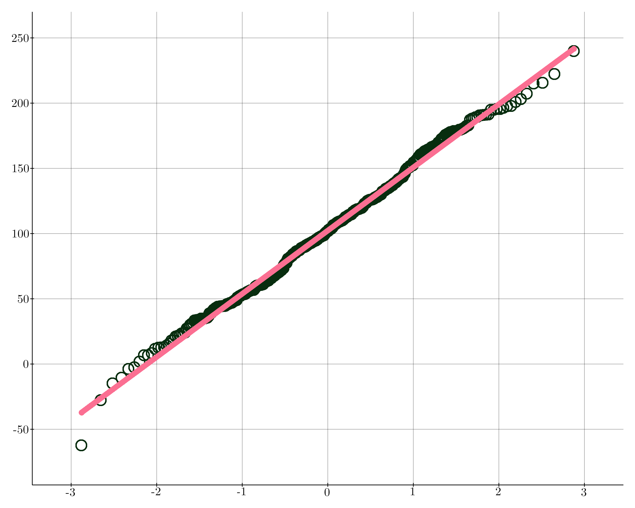
QQ plot

import kaxe

data = [1.2, 0.8, 1.5, 0.3, 2.1, -0.4, 0.9]
qq = kaxe.QQPlot(data)
qq.save("qq.png")

class kaxe.QQPlot(data, quantiles: list = None, color: list = [None, None], size=50)

Bases: BoxedPlot

Initialize a QQPlot instance.

Parameters:

data (list) – The data points to be plotted on the QQ plot.
quantiles (list, optional) – The theoretical quantiles to compare against. If not provided, standard normal quantiles are calculated based on the length of data.
color (list, optional) – A list containing two color values for the plot. Defaults to [None, None]. If None, a random color is generated.
size (int, optional) – The size of the points in the plot. Default is 50.

points

The 2D points object representing the data and quantiles.

Type:: Points2D

line

The 2D function represeting an line

Type:: Function2D

Notes

A linear fit is applied to the data and quantiles, and the resulting line is added to the plot.