Plots

All plots inherits from the Window base class. This class should not be used in practise and is only used to be inherited from.

class kaxe.Window

Bases: AttrObject

The main window class that handles the rendering and layout of graphical elements.

It manages padding, styles, and the inclusion of various elements such as shapes and legends. The window can be rendered and saved as an image, and it supports different terminal types including Jupyter and IPython.

AttrMap.style(styles: dict = {}, **kstyles)

Set multiple styles for the object.

Parameters:

styles (dict, optional) – A dictionary of styles to set. Default is an empty dictionary.
**kstyles (keyword arguments) – Additional styles to set as keyword arguments.

Examples

>>> plt.style(color=(255,0,0,255), fontSize=128)
>>> plt.style({'marker.tickWidth': 10}, fontSize=64)

Paramaters

obj: Object to be added to the plot

Examples

>>> plt.add(kaxe.Function( ... ))
>>> plt.add(kaxe.Points( ... ))

adjust(procentWidth, documentFontSize=0.25, documentMarginProcent=1.5, documentWidth=11.8, imageSlimRatio=1)

Adjust the following styles based on document size and document font size. i. e. match document font size with plot font size

Directly changed styles; fontSize, width, height, outerPadding, xNumbers, yNumbers

A lot of styles indirecitly relies on fontSize, width and height.

Resources

https://paper-size.com/c/a-paper-sizes.html https://www.overleaf.com/learn/latex/Page_size_and_margins#Paper_size,_orientation_and_margins https://tex.stackexchange.com/questions/272607/what-is-the-name-of-latexs-default-style-and-why-was-it-chosen-for-latex https://tex.stackexchange.com/questions/155896/what-is-the-default-font-size-of-a-latex-document https://tex.stackexchange.com/questions/8260/what-are-the-various-units-ex-em-in-pt-bp-dd-pc-expressed-in-mm

getVisualScale(): Scale factor for visual elements (points, line widths). 1.0 for normal plots; >1 when zoomed in.

save(fname: str | BytesIO, format: str | None = None, *, project: str | None = None)

Save the current window image to a file.

If a cached image is available, it will be used to save the file. Otherwise, the image will be generated and then saved.

Parameters:

fname (str | BytesIO) – The filename where the image will be saved or a BytesIO object to save the image in memory.
format (str, optional) – Output format: "png", "svg", or "pdf". Inferred from fname extension when omitted.
project (str, optional) – If given, also write a .kaxe JSON project file to this path (editable figure source).

Examples

>>> plt.save( path/where/image/saved.png )
>>> plt.save( path/where/image/saved.svg )
>>> plt.save( path/where/image/saved.pdf )

show()

Show the current image using Pillow.Image.Show

If a cached image is available, it will be used to save the file. Otherwise, the image will be generated and then saved.

Examples

>>> plt.show( )

theme(theme)

Applies a theme to the window by updating its style attributes.

Parameters:: theme (dict) – A dictionary containing style attributes and their values.

Examples

>>> plt.theme(kaxe.Themes.A4Medium)

Export

See Export and Display for PNG, SVG, and Jupyter display details.

Classical Plot

class kaxe.Plot(window: list = None)

Bases: Window

A simple plotting window for cartesian coordinates

firstAxis

The first axis of the plot.

Type:: Kaxe.Axis

secondAxis

The second axis of the plot.

Type:: Kaxe.Axis

Parameters:: window (list) – A list representing the axis window [x0, x1, y0, y1].

Examples

>>> import kaxe
>>> plt = kaxe.Plot()
>>> plt.add( ... )
>>> plt.show( )

pad(x=0, y=None, *, relative=False, percent=False)

Expand the data window symmetrically on each axis (after bounds are resolved).

Default is absolute padding in the same units as the axes. With relative=True, x and y are fractions of each axis span: the amount added on the low and high side is fraction * (max - min), so pad(0.1, relative=True) widens x by 20% of the original x span (10% on each side). With percent=True, the same rule applies but x/y are percents (pad(10, percent=True) equals pad(0.1, relative=True)).

Relative padding is applied first, then absolute, if you set both.

For DoubleAxisPlot, y uses each y scale’s own span when relative.

Parameters:

x (float, optional) – Padding for x (absolute units, span fraction, or percent). Default 0.
y (float, optional) – Padding for y (and both y scales on a double-axis plot). If omitted, uses x.
relative (bool, optional) – If True, x/y are fractions of the axis span(s). Default False.
percent (bool, optional) – If True, x/y are percents of the span (implies relative). Default False.

Examples

>>> plt.pad(0.05)
>>> plt.pad(0.1, relative=True)
>>> plt.pad(5, percent=True)

title(first=None, second=None)

Adds title to the plot.

Parameters:

first (str, optional) – Title for the first axis.
second (str, optional) – Title for the second axis.

Returns:

The active plotting window

Return type:

Kaxe.Plot

zoom(x0: float = None, x1: float = None, y0: float = None, y1: float = None, position: str = 'top-left', size: tuple = (400, 300), showAxes: bool = True, connectorLines: bool = True, connectorCorners: str = 'auto', includeMain: bool = True, margin: int = 20, selectionBoxWidth: int = 3, selectionBoxColor: tuple = (0, 0, 0, 255), connectorWidth: int = 2, connectorColor: tuple = (0, 0, 0, 255))

Create a zoom inset (magnifying glass) showing a magnified view of a region. Returns a linked subplot where objects added via zoom.add() appear only in the inset.

Parameters:

x0 (float) – Data coordinates of the zoom region. Can also pass as zoom([x0, x1, y0, y1]).
x1 (float) – Data coordinates of the zoom region. Can also pass as zoom([x0, x1, y0, y1]).
y0 (float) – Data coordinates of the zoom region. Can also pass as zoom([x0, x1, y0, y1]).
y1 (float) – Data coordinates of the zoom region. Can also pass as zoom([x0, x1, y0, y1]).
position (str or tuple, optional) – Preset: ‘top-left’, ‘top-right’, ‘bottom-left’, ‘bottom-right’. Or (x, y) in data coordinates for the bottom-left corner of the inset. Default ‘top-left’.
size (tuple, optional) – (width, height) of inset in pixels. Default (400, 300).
showAxes (bool, optional) – Whether to show axes in the inset. Default True.
connectorLines (bool, optional) – Whether to draw connector lines. Default True.

Returns:

Plot-like object with .add() for inset-only content.

Return type:

ZoomInset

Examples

>>> zoom = plt.zoom(620, 740, 4.4, 5.2)
>>> zoom.add(kaxe.Points2D([680], [4.8]))

Zoom inset

Use kaxe.Plot.zoom() to add a magnified region with optional connector lines. The returned inset accepts its own objects via zoom.add():

import math
import kaxe

plot = kaxe.Plot([0, 4 * math.pi, -1, 1])
plot.add(kaxe.Function2D(math.sin))
zoom = plot.zoom(2.5, 4, -0.4, -0.1, position=(5, -0.5))
zoom.add(kaxe.Points2D([3.2], [-0.2], color=(255, 0, 0, 255)))

class kaxe.BoxedPlot(window: list | tuple | None = None)

Bases: Plot

A class used to create a plot where the axis is always to the left and at the bottom.

firstAxis

The first axis of the plot.

Type:: Kaxe.Axis

secondAxis

The second axis of the plot.

Type:: Kaxe.Axis

Parameters:: window (list|tuple|None, optional) – A list or tuple defining the window for the plot, by default None.

class kaxe.EmptyPlot(window: list | tuple | None = None)

Bases: Plot

A almost empty plotting window. Axis have no numbers

firstAxis

The first axis of the plot.

Type:: Kaxe.Axis

secondAxis

The second axis of the plot.

Type:: Kaxe.Axis

Parameters:: window (Union[list, tuple, None], optional) – The window configuration for the plot. Default is None.

class kaxe.EmptyWindow(window: list | tuple | None = None)

Bases: Plot

A completely empty plotting window.

firstAxis

The first axis of the plot.

Type:: Kaxe.Axis

secondAxis

The second axis of the plot.

Type:: Kaxe.Axis

Parameters:: window (Union[list, tuple, None], optional) – The window configuration for the plot. Default is None.

Note

Yes, its blank

class kaxe.DoubleAxisPlot(window: list | tuple | None)

Bases: Plot

A plotting window with two y-axis placed on each end of axis

firstAxis

The first axis of the plot.

Type:: Kaxe.Axis

secondAxis

The second axis of the plot.

Type:: Kaxe.Axis

Parameters:: window (list|tuple|None) – [x0, x1, ya0, ya1, yb0, yb1], A list or tuple defining the window for the plot The first two values are the x-axis window, the next two are the first y-axis window, and the last two are the second y-axis window.

Note

This plot window is still in early devolplement

add1(obj)

Adds to the first Axis

Parameters:: object (Object) – The object to add to the left axis

add2(obj)

Adds to the first Axis

Parameters:: object (Object) – The object to add to the second axis

title(first=None, second=None, third=None)

Adds title to the plot.

Parameters:

first (str, optional) – Title for the first axis.
second (str, optional) – Title for the second axis.
third (str, optional) – Title for the second second axis. Called the third axis

Returns:

The active plotting window

Return type:

Kaxe.Plot

Polar plot

class kaxe.PolarPlot(window: list = None, useDegrees: bool = False)

Bases: Window

A polar plot with radians on the radial axis

radiusAxis

The radial axis of the polar plot.

Type:: Kaxe.Axis

Note

This plotting window supports fewer objects than that of the classical plotting windows

title(title: str)

Adds title to the plot.

Parameters:: title (str) – Title for the axis.
Returns:: The active plotting window
Return type:: Kaxe.Plot

Logarithmic Plot

class kaxe.LogPlot(window: list = None, firstAxisLog=False, secondAxisLog=True, hideUgly=True)

Bases: Plot

LogPlot class for creating logarithmic plots.

firstAxis

The first axis of the plot.

Type:: Kaxe.Axis

secondAxis

The second axis of the plot.

Type:: Kaxe.Axis

Parameters:

window (list, optional) – A list defining the axis window as [x0, x1, y0, y1]. Default is None.
firstAxisLog (bool, optional) – If True, the first axis (x-axis) will be logarithmic. Default is False.
secondAxisLog (bool, optional) – If True, the second axis (y-axis) will be logarithmic. Default is True.
hideUgly (bool, optional) – If True, hides markers that are not round numbers in logarithmic scale. Default is True.

class kaxe.BoxedLogPlot(window=None, firstAxisLog=False, secondAxisLog=True, hideUgly=True)

Bases: LogPlot

BoxLogPlot class for creating logarithmic plots with axis placed at borders.

firstAxis

The first axis of the plot.

Type:: Kaxe.Axis

secondAxis

The second axis of the plot.

Type:: Kaxe.Axis

Parameters:

window (list, optional) – A list defining the axis window as [x0, x1, y0, y1]. Default is None.
firstAxisLog (bool, optional) – If True, the first axis (x-axis) will be logarithmic. Default is False.
secondAxisLog (bool, optional) – If True, the second axis (y-axis) will be logarithmic. Default is True.
hideUgly (bool, optional) – If True, hides markers that are not round numbers in logarithmic scale. Default is True.

3D Plots

Caution

Kaxe 3D graphs are pretty, but are still in early devolplement. Also Kaxe is written enterily in Python and is thereby slow. This method should in the future utilize the GPU, but for the time being this methods relies enterily on the CPU to create the graphs.

class kaxe.Plot3D(window: list = None, rotation: list | tuple = [60, -70], size: bool | list | tuple = None, drawBackground: bool = False, light: list = [0, 0, 0], addMarkers: bool = True)

Bases: Plot3DAxesMixin, Window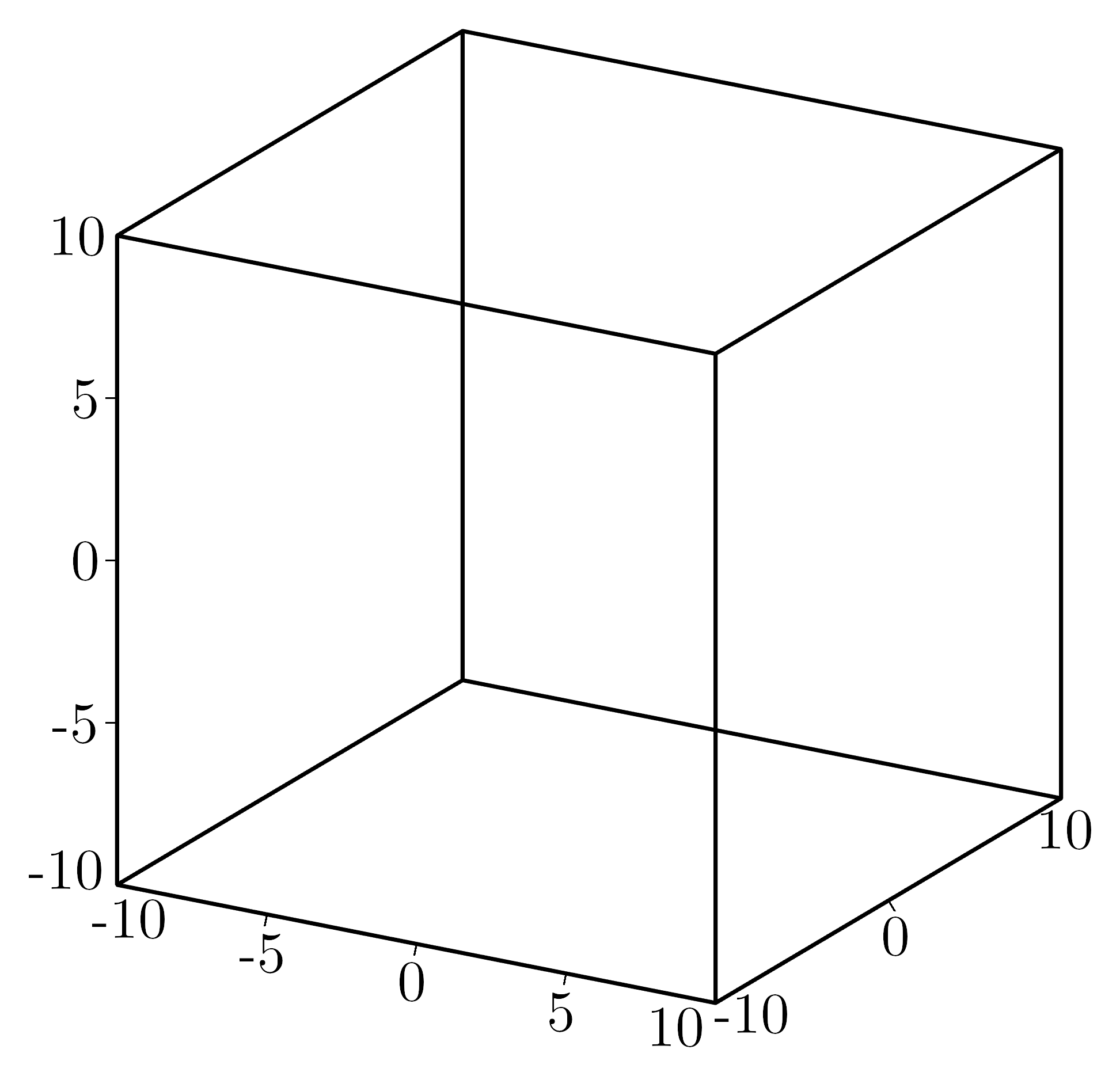

inside(x, y, z=None): para: translated (pixels)

inversetranslate(x: int, y: int): para: translated value return: x,y position according to basis (1,0), (0,1) in abstract space

pixel(x: int, y: int, z: int) → tuple

Transform user coordinates to final 3D render coordinates.

This is the main coordinate transformation function used throughout the plotting system. It scales user data coordinates and applies the cube centering offset.

Parameters:

x (int) – Coordinates in user data space
y (int) – Coordinates in user data space
z (int) – Coordinates in user data space

Returns:

Final 3D coordinates ready for rendering

Return type:

tuple

save(fname: str | BytesIO, format: str | None = None, *, project: str | None = None)

Save the current window image to a file.

If a cached image is available, it will be used to save the file. Otherwise, the image will be generated and then saved.

Parameters:

fname (str | BytesIO) – The filename where the image will be saved or a BytesIO object to save the image in memory.
format (str, optional) – Output format: "png", "svg", or "pdf". Inferred from fname extension when omitted.
project (str, optional) – If given, also write a .kaxe JSON project file to this path (editable figure source).

Examples

>>> plt.save( path/where/image/saved.png )
>>> plt.save( path/where/image/saved.svg )
>>> plt.save( path/where/image/saved.pdf )

scaled3D(x: int, y: int, z: int) → tuple

Transform user coordinates to normalized 3D space.

Converts from user data coordinates to the normalized cube space used internally by the 3D renderer. Each axis is independently scaled according to the plot bounds and size ratios.

Parameters:

x (int) – Coordinates in user data space
y (int) – Coordinates in user data space
z (int) – Coordinates in user data space

Returns:

Coordinates in normalized 3D space [-0.5*size, +0.5*size]

Return type:

tuple

show(gui=True)

Show the current image using Pillow.Image.Show

If a cached image is available, it will be used to save the file. Otherwise, the image will be generated and then saved.

Examples

>>> plt.show( )

supports_vector_export = False

A 3D plotting window with full wireframe box and automatic axis positioning.

This class provides a complete 3D plotting environment with: - Automatic wireframe box generation around the plot volume - Dynamic axis positioning based on camera angle for optimal visibility - OpenGL-accelerated rendering with lighting support - Interactive rotation and real-time manipulation - Background grid lines and face highlighting

The coordinate system follows right-hand rule with: - X-axis: left-right (red lines in debug mode) - Y-axis: front-back (green lines in debug mode) - Z-axis: up-down (blue lines in debug mode)

Rendering Pipeline: 1. Setup camera and 3D transformations (__before__) 2. Generate wireframe box geometry (__createWireframe__) 3. Calculate visible faces and axis positions (__after__) 4. Position axes on closest visible edges to camera 5. Add grid lines and background faces 6. Render all 3D objects to 2D image

axis

The three axes of the plot [x_axis, y_axis, z_axis]

Type:: list[Axis]

render

The 3D rendering engine instance

Type:: OpenGLRender

rotation

Current camera rotation angles [alpha, beta] in degrees

Type:: list[float]

light

Light direction vector [x, y, z]. Zero vector disables lighting

Type:: list[float]

windowAxis

Plot bounds [x_min, x_max, y_min, y_max, z_min, z_max]

Type:: list[float]

Parameters:

window (list, optional) – The plot bounds [x0, x1, y0, y1, z0, z1] (default: [-10, 10, -10, 10, -10, 10])
rotation (list, optional) – Camera angles [alpha, beta] in degrees (default: [60, -70])
size (list | bool | None, optional) – Axis scaling: True for automatic, list for custom ratios, None for unit cube
drawBackground (bool, optional) – Whether to draw background faces and grid lines (default: False)
light (list, optional) – Light direction vector [x, y, z] (default: [0, 0, 0] = no lighting)
addMarkers (bool, optional) – Whether to add tick marks and labels to axes (default: True)

Notes

The plot automatically selects the best axis positioning based on camera angle to avoid overlapping lines and ensure maximum visibility. The wireframe box consists of 12 edges forming a cube, with axes positioned on the 3 most visible edges closest to the camera.

title(firstAxis=None, secondAxis=None, thirdAxis=None)

Adds title to the plot.

Parameters:

firstAxis (str, optional) – Title for the first axis.
secondAxis (str, optional) – Title for the second axis.
thirdAxis (str, optional) – Title for the third axis.

Returns:

The active plotting window

Return type:

Kaxe.Plot

class kaxe.PlotCenter3D(window: list = None, rotation=[60, -70], size: bool | list | tuple = None, light: list = [0, 0, 0], addMarkers: bool = True)

Bases: Plot3D

A plotting window used to represent a 3D Plot with axis placed correctly

Parameters:

window (list, optional) – The window dimensions for the plot in the format [x0, x1, y0, y1, z0, z1] (default is [-10, 10, -10, 10, -10, 10]).
rotation (list, optional) – The rotation angles for the plot in degrees [alpha, beta] (default is [60, -70]).
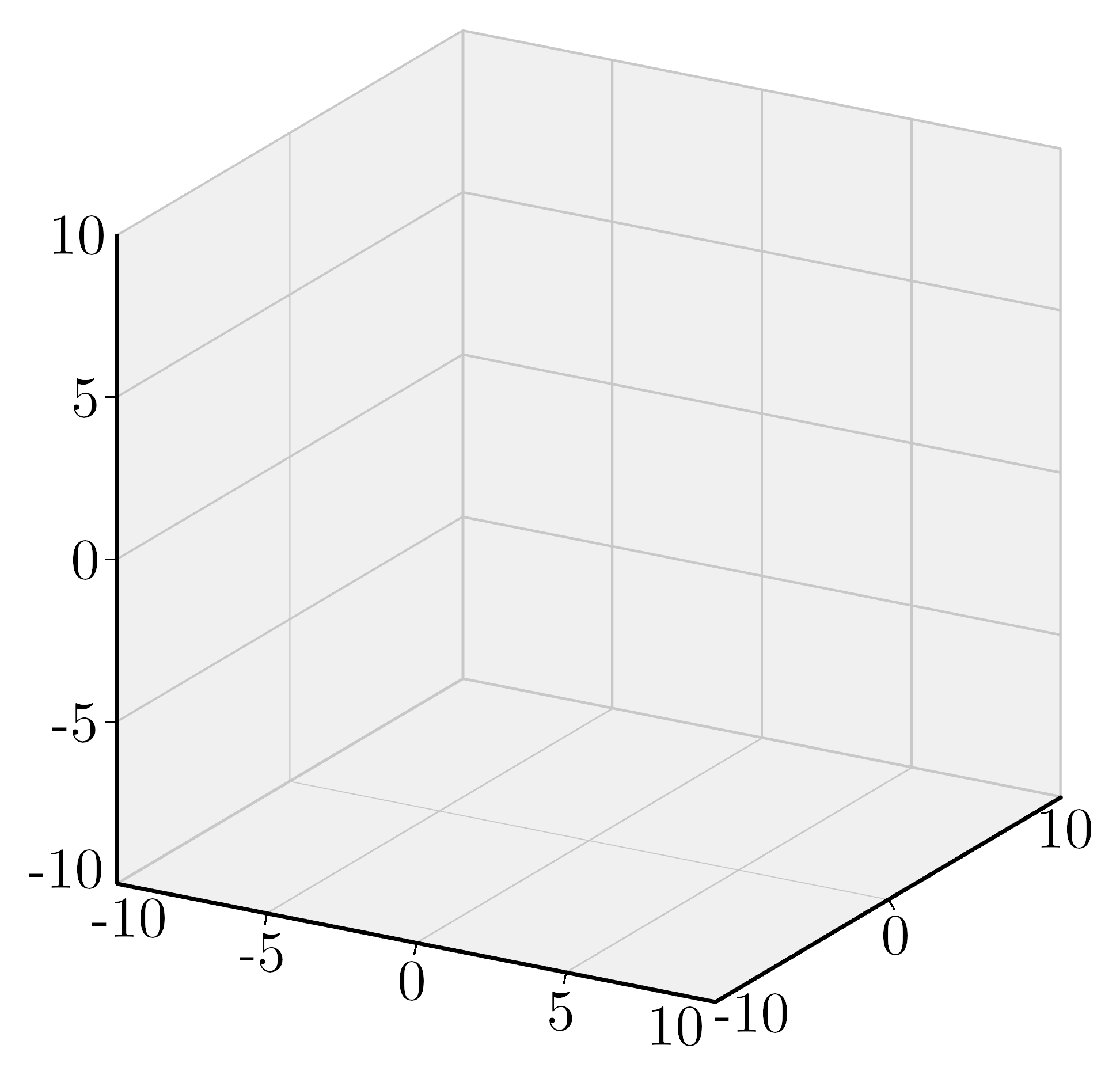
drawBackground (bool, optional) – Draw background with gridlines
size (list | bool | None, optional) – if True the axis will be scaled accordingly to window. If a list is passed theese sizes will be used.
light (list, optional) – light direction. If null vector is given light will not be added.

class kaxe.PlotFrame3D(window: list = None, rotation=[60, -70], drawBackground=True, size: bool | list | tuple = None, light: list = [0, 0, 0])

Bases: Plot3D

A plotting window used to represent a 3D Plot with only x-, y- and z-axis drawn

Parameters:

window (list, optional) – The window dimensions for the plot in the format [x0, x1, y0, y1, z0, z1] (default is [-10, 10, -10, 10, -10, 10]).
rotation (list, optional) – The rotation angles for the plot in degrees [alpha, beta] (default is [0, -20]).
size (list | bool | None, optional) – if True the axis will be scaled accordingly to window. If a list is passed theese sizes will be used.
light (list, optional) – light direction. If null vector is given light will not be added.

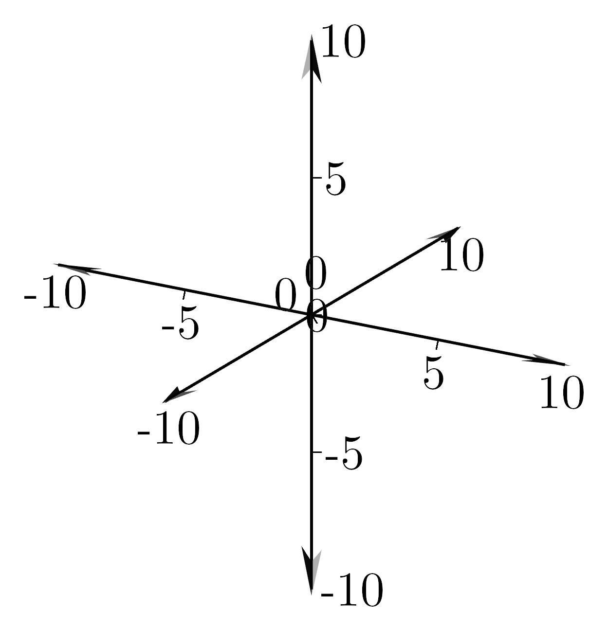
class kaxe.PlotEmpty3D(window: list = None, rotation=[60, -70], size: bool | list | tuple = None, light: list = [0, 0, 0])

Bases: Plot3D

A plotting window used to represent a 3D Plot without axis drawn

Parameters:

window (list, optional) – The window dimensions for the plot in the format [x0, x1, y0, y1, z0, z1] (default is [-10, 10, -10, 10, -10, 10]).
rotation (list, optional) – The rotation angles for the plot in degrees [alpha, beta] (default is [0, -20]).
size (list | bool | None, optional) – if True the axis will be scaled accordingly to window. If a list is passed theese sizes will be used.
light (list, optional) – light direction. If null vector is given light will not be added.

Note

This one is also just empty

Grid

Combine multiple plot windows into one image. Sub-plots keep their own styles and objects:

import kaxe

top = kaxe.Plot([-3, 3, -3, 3])
top.add(kaxe.Function2D(lambda x: x))

bottom = kaxe.Plot([-3, 3, -3, 3])
bottom.add(kaxe.Function2D(lambda x: x**2))

grid = kaxe.Grid()
grid.addColumn(top, bottom)
grid.save("stacked.png")

Use addRow(*plots) for horizontal layouts. kaxe.Grid saves PNG only — see Export and Display.

class kaxe.Grid

Bases: AttrObject

Assemble multiple plots in one image.

Examples

>>> grid = kaxe.Grid()
>>> grid.style(width=500, height=500)
>>> grid.addRow(plt1, plt2)
>>> grid.addColumn(plt3, plt4)
>>> grid.show()
>>> grid.save('fname.png')
>>> grid.save('fname.svg')  # 2D vector; 3D cells embed as raster
>>> grid.save('fname.pdf')  # 2D vector PDF; requires kaxe[pdf]

addColumn(*column: list)

Adds a column of plots to the grid.

Parameters:: column (list) – A list of plots to be added as a column in the grid.

addRow(*row: list)

Adds a row of plots to the grid.

Parameters:: row (list) – A list of plots to be added as a row in the grid.

adjust(procentWidth, documentFontSize=0.25, documentMarginProcent=1.5, documentWidth=11.8, imageSlimRatio=1)

Adjust grid size and typography for LaTeX page fractions (same API as kaxe.Plot.adjust()).

Sets width, height, fontSize, outerPadding, and per-cell xNumbers / yNumbers from cell size. zNumbers is set when the grid contains 3D plots.

See kaxe.core.window.Window.adjust() for parameter details.

legends(*legends)

Set the legends for the grid. All information must be provided for a legend.

Parameters:: *legends (list[tuple]) – Diffrent legends consisting of a label, color and symboltype

Examples

>>> grid.legends(
    ("A legend", kaxe.Symbol.CROSS, color1),
    ...
    ("N legend", kaxe.Symbol.CIRCLE, colorn),
)

show()

Show the current image using Pillow.Image.Show

If a cached image is available, it will be used to save the file. Otherwise, the image will be generated and then saved.

Examples

>>> plt.show( )

theme(theme): Apply a theme dict (e.g. kaxe.Themes.A4Medium) to the grid.